Deep Q-Networks
In this article, we will learn about Deep Q-Networks and a basic implementation of it.
Recap
Q-Learning and some Formal Definitions
What is a Policy?
We can define policy as a mapping from states to actions, its the objective in reinforcement learning to find the optimal policy, which is defined as the policy which maximises the return.
Return / Future Total Reward
We define return as the sum of all immediate rewards on a particular episode, ie, the sum of rewards up until the episode finish.
Future Discounted Reward
We add to our total reward a parameter called gamma ( ). If = 0, all future rewards will be discarded otherwise they will be considered. We can interpret this parameter as in terms of how much we value our future rewards compared to our current reward.
What is an Episode?
Our environment is based on an MDP (Markov Decision Process) which means that our state encodes everything needed to take a decision by defining an episode as a finite set of states, actions and rewards. Here, we get a reward taking the action from a state and an episode always finishes on an end/final state.
Q function
We define the function as maximum expected return that we can get if we take an action on state , and continue from that point until the end of the episode which means that we continue choosing actions from the policy derived from Q.
Below we see how the Q function, basically updates to give the biggest Q value on state . Every time an action is taken we update its Q-value:
Here is the learning rate and is the discount factor.
Greedy policy
If we choose an action that simply maximizes the return every time, this causes a problem. It becomes a pure greedy algorithm and prevents exploration from happening which may give you better options of finding better actions. This is called exploration-exploitation problem and to solve this we use an algorithm called Epsilon Greedy Algorithm, where a small probability will choose a completely random action from time to time.
Deep Q-Networks
| DQN |
|---|
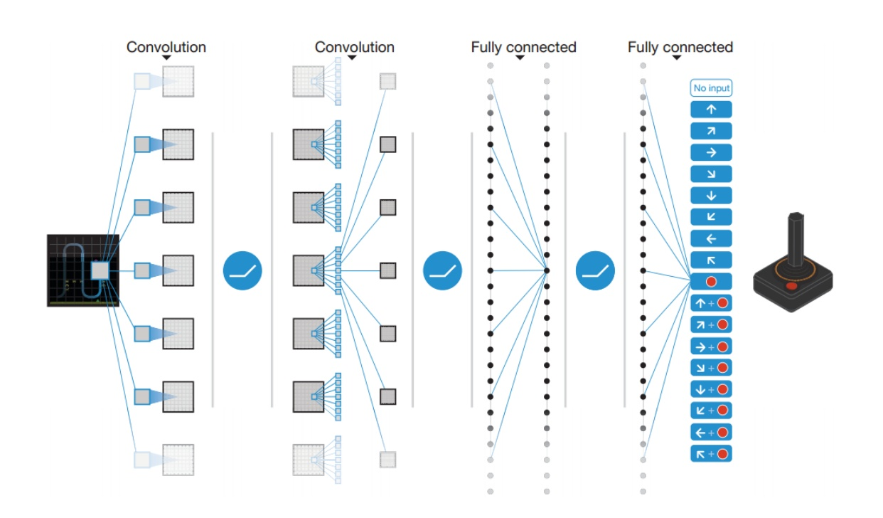 |
A Deep Q Neural Network, instead of using a Q-table, a Neural Network basically takes a state and approximates Q-values for each action based on that state. This involves parametrizing the Q values.
To explain further, tabular Q-Learning creates and updtaes a Q-Table, given a state, to find maximum return. This is however not scalable, and hence we need an efficient way for Q-Learning to function in an environment with many states and actions. The best idea in this case is to create a neural network that will approximate, given a state, the different Q-values for each action.
| Difference between Q-Learning and DQN |
|---|
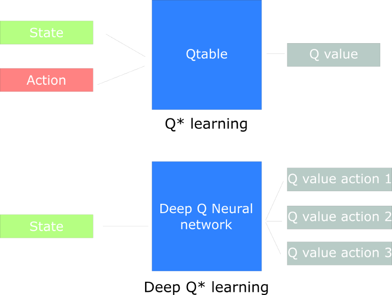 |
Here, our model will still implement the same Bellman Equation, but here the Neural Network updates the weights by taking the difference between our Q_target (maximum possible value from the next state) and Q_value (our current prediction of the Q-value) in order to reduce the errors in weights.
And, we have our Loss Function as the Squared Error between target Q-value and the Q-value output from the network.
Convolutional Layers
If our agent is going to be learning to play certain games, it has to be able to make sense of the game’s screen output, and instead of considering each pixel independently, convolutional layers allow us to consider regions of an image and maintain spatial relationships between the objects on the screen as we send information up to higher levels of the network. In this way, they act similarly to how humans percieve the screen. Hence, they are ideal for the first few elements within our network.
Experience Replay
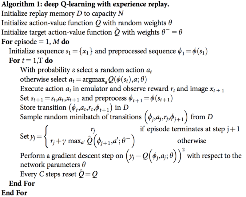
The idea of Experience Replay is that by storing an agent’s experiences, and randomly drawing batches of them to train the network, we can more robustly learn to perform well in the task. By keeping the experiences we draw random, we prevent the network from only learning about what it was immediately doing in the environment, and allow it to learn from many of it’s past experiences as well. Each of these experiences are stored as tuples of [ state , action , reward , next state ]. The Experience Replay buffer stores a fixed number of recent memories, and as new ones come in, old ones are removed. When the time comes to train, we simply draw a uniform batch of these random memories from the buffer, and train our network with them.
Separate Target Network
DQNs utilize a second network during the training procedure. This second network is used to generate the target-Q values that will be used to compute the loss for every action during training. One may ask, why not use just use one network for both estimations? An issue arises that at every step of training, the Q-network’s values shift, and if we are using a constantly shifting set of values to adjust our network values, then the value estimations can easily go out of control and cause errors in calculation.
The network can become destabilized by falling into feedback loops between the target and estimated Q-values. In order to prevent this risk, the target network’s weights are fixed, and only updated periodically to the primary Q-networks values. In this way, training happens in a stable manner.
Here is the complete DQN Algorithm with Experience Replay:
| DQN Algorithm |
|---|
 |
Implementation
Here we will be implementing a basic cartpole environment which uses DQN. First, we call the required libraries and set our hyper parameters for our models, and configure if we will be using a GPU or not.
import gym
from gym import wrappers
import random
import math
import torch
import torch.nn as nn
import torch.optim as optim
from torch.autograd import Variable
import torch.nn.functional as F
import matplotlib.pyplot as plt

# hyper parameters
EPISODES = 200  # number of episodes
EPS_START = 0.9  # e-greedy threshold start value
EPS_END = 0.05  # e-greedy threshold end value
EPS_DECAY = 200  # e-greedy threshold decay
GAMMA = 0.8  # Q-learning discount factor
LR = 0.001  # NN optimizer learning rate
HIDDEN_LAYER = 256  # NN hidden layer size
BATCH_SIZE = 64  # Q-learning batch size

# if gpu is to be used
device = torch.device("cuda" if torch.cuda.is_available() else "cpu")
use_cuda = torch.cuda.is_available()
FloatTensor = torch.cuda.FloatTensor
LongTensor = torch.cuda.LongTensor
ByteTensor = torch.cuda.ByteTensor
Tensor = FloatTensor
Replay Memory and Network Definitions are given below, here, we do not use a convolutional network to load the rendered images, but instead we load the actions (observation values) from the environment. The network uses a simple NN with linear hidden layers. Replay Memory here is a cyclic buffer of bounded size that holds the transitions observed recently, and we also have random.sample() function which is called to select random batches of transitions for training.
class ReplayMemory:
    def __init__(self, capacity):
        self.capacity = capacity
        self.memory = []

    def push(self, transition):
        self.memory.append(transition)
        if len(self.memory) > self.capacity:
            del self.memory[0]

    def sample(self, batch_size):
        return random.sample(self.memory, batch_size)

    def __len__(self):
        return len(self.memory)


class Network(nn.Module):
    def __init__(self):
        nn.Module.__init__(self)
        self.l1 = nn.Linear(4, HIDDEN_LAYER)
        self.l2 = nn.Linear(HIDDEN_LAYER, 2)

    def forward(self, x):
        x = F.relu(self.l1(x))
        x = self.l2(x)
        return x
Now we can specify the environment being used, that is the cartpole environment and set the optimizer as well (we use the Adam optimizer here).
env = gym.make('CartPole-v0')
env = wrappers.Monitor(env, './tmp/cartpole-v0-1')

model = Network()
if use_cuda:
    model.cuda()
memory = ReplayMemory(10000)
optimizer = optim.Adam(model.parameters(), LR)
steps_done = 0
episode_durations = []
Now we can instantiate our model and its optimizer, and define some utilities required. The select_action() function selects an action accordingly to an epsilon greedy policy, so we either use our model for choosing the action or just sample one uniformly. The probability of choosing a random action will start at EPS_START and will decay exponentially towards EPS_END. EPS_DECAY controls the rate of the decay.
plot_durations() is simply a helper function for plotting the durations of episodes, along with an average over the last 100 episodes.
Our Learn function specified below will load a random batch from the experience replay memory and calculates the current and next Q values for all actions taken now, (highet for those actions that will have to be taken) and computes loss and also backpropagates the loss in the network.
def select_action(state):
    global steps_done
    sample = random.random()
    eps_threshold = EPS_END + (EPS_START - EPS_END) * math.exp(-1. * steps_done / EPS_DECAY)
    steps_done += 1
    if sample > eps_threshold:
        return model(Variable(state, volatile=True).type(FloatTensor)).data.max(1)[1].view(1, 1)
    else:
        return LongTensor([[random.randrange(2)]])


def run_episode(e, environment):
    state = environment.reset()
    steps = 0
    while True:
        environment.render()
        action = select_action(FloatTensor([state]))
        next_state, reward, done, _ = environment.step(action[0, 0])

        # negative reward when attempt ends
        if done:
            reward = -1

        memory.push((FloatTensor([state]), action,  # action is already a tensor
                    FloatTensor([next_state]), FloatTensor([reward])))
        learn()

        state = next_state
        steps += 1

        if done:
            print("{2} Episode {0} finished after {1} steps"
                  .format(e, steps, '\033[92m' if steps >= 195 else '\033[99m'))
            episode_durations.append(steps)
            plot_durations()
            break


def learn():
    if len(memory) < BATCH_SIZE:
        return

    # random transition batch is taken from experience replay memory
    transitions = memory.sample(BATCH_SIZE)
    batch_state, batch_action, batch_next_state, batch_reward = zip(*transitions)

    batch_state = Variable(torch.cat(batch_state))
    batch_action = Variable(torch.cat(batch_action))
    batch_reward = Variable(torch.cat(batch_reward))
    batch_next_state = Variable(torch.cat(batch_next_state))

    # current Q values are estimated by the network for all actions
    current_q_values = model(batch_state).gather(1, batch_action)
    # expected Q values are estimated from actions which gives maximum Q value
    max_next_q_values = model(batch_next_state).detach().max(1)[0]
    expected_q_values = batch_reward + (GAMMA * max_next_q_values)

    # loss is measured from error between current and newly expected Q values
    loss = F.smooth_l1_loss(current_q_values, expected_q_values)

    # backpropagation
    optimizer.zero_grad()
    loss.backward()
    optimizer.step()


def plot_durations():
    plt.figure(2)
    plt.clf()
    durations_t = torch.FloatTensor(episode_durations)
    plt.title('Training...')
    plt.xlabel('Episode')
    plt.ylabel('Duration')
    plt.plot(durations_t.numpy())
    # take 100 episode averages and plot them too
    if len(durations_t) >= 100:
        means = durations_t.unfold(0, 100, 1).mean(1).view(-1)
        means = torch.cat((torch.zeros(99), means))
        plt.plot(means.numpy())

    plt.pause(0.001)  # pause a bit so that plots are updated
Now, we can call the episodes based on the number of episodes specified, it is encouraged to tweak this value to higher numbers to observe how DQN converges after a certain number of episodes.
for e in range(EPISODES):
    run_episode(e, env)

print('Complete')
env.render(close=True)
env.close()
plt.ioff()
plt.show()
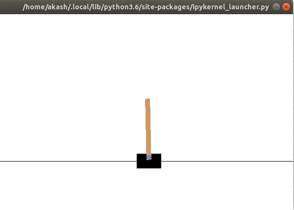
And we get a pretty decent score in the environment depending on the number of episodes you run. It is said to converge around 700-800 or so episodes for DQNs.
| Cartpole Output |
|---|
 |
Conclusion
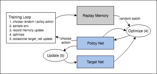
Hence DQNs have been covered along a with a beginner implementation on pyTorch. Just in case there is confusion in how the data flow occurs within the model, it is worth visiting this diagram provided in the pyTorch documentation for DQNs, which clearly show how the updates are made.
| DataFlow |
|---|
 |