Deep Recurrent Q-Network
In this article, we will learn about Deep recurrent Q-learning and POMDP and find out why DRQN works better in case of POMDP than DQN.
MDP vs. POMDP (Partially Observable MDP)
In an MDP we have full knowledge of the environment. But in most of the cases, it is not possible to know the complete state of the environment. Like a single game screen is not sufficient to determine the state of the system. For example, have a look at the picture below -

Just by looking at one image we cannot say whether the girl passed the ball and the boy is trying to catch it or vice versa. Therefore we only have partial knowledge of the environment, and this is the case most of the time. Thus for our agent to learn a policy in a POMDP where instead of entire information about the current state only an observation of the current state is available, we need to use a different method, a method such that our agent automatically can remember what it has seen in past and can learn a policy.
Why DRQN and not DQN for POMDPs?
In the DQN algorithm, we had to stack frames together to get complete information of the current state as depicted by the images below-

With four pictures together we can make out in which direction the ball is moving, it can also help in having a sense of velocity of the moving object. According to the DRQN Paper for Atari 2600 games, stacking four frames together makes all the games an MDP. But for more complex environments stacking four frames together may not be enough. The agent may need to remember something that happened many time steps ago to understand the current state. In that case, i.e., in case of such POMDPs DRQN works better than DQN.
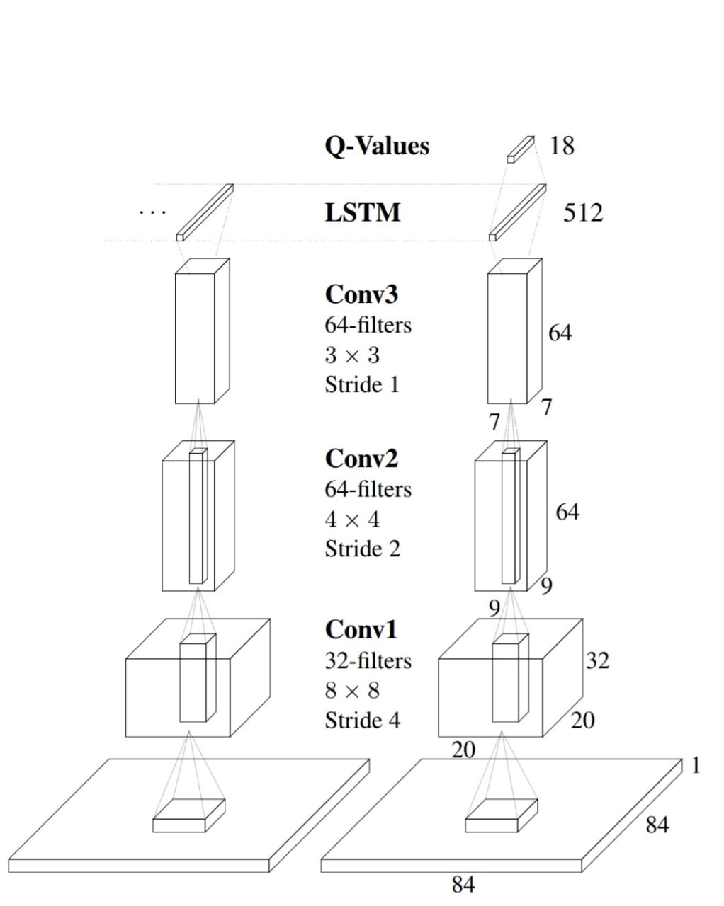
In DRQN the first fully connected layer of DQN is replaced by an LSTM(Long Short Term Memory network) layer. If you do not know about LSTMs, refer to this blog post. Recurrent neural networks can remember information from several time steps before and thus LSTMs are used. This is why DRQNs can learn even if single game screens are passed one by one, and hence they work better than DQN in case of POMDPs.
Following is the DRQN architecture used in the original paper.
Implementation Details
Here, I am listing down some of the important points to be taken care of while implementing DRQN. For more details refer the DRQN Paper.
-
LSTM’s hidden state must be set to zero at the start of each update. However, this makes it hard for LSTM to learn functions that span over longer timescales.
-
Stable recurrent updates
-
Bootstrapped Sequential Updates
- In this, the episodes are selected randomly from the replay memory, and updates proceed from the beginning of the episode to the end of it. The RNNs hidden state is carried forward throughout the episodes.
-
Bootstrapped Random Updates
- Episodes are selected randomly from the replay memory, and updates start at a random point in the episode and continue for a certain number of time steps.
-
-
Both sequential updates and random updates yield convergent policies and hence any of them can be used.
Let’s go through the code and understand the implementation step by step.
1.Import the necessary libraries.
import random
import math
import gym
import numpy as np
import PIL
from PIL import Image
import matplotlib
import matplotlib.cm as cm
import torch
import torch.nn as nn
import torch.optim as optim
import torch.nn.functional as F
import torchvision.transforms as T
2.In this step, we will make our DRQN model, the convolutional layer sizes and all other hyperparameters are according to the original paper.
class model(nn.Module):
def __init__(self):
super(model,self).__init__()
self.hidden_size = 512
self.conv1=nn.Conv2d(4,32,kernel_size=8,stride=4)
self.bn1=nn.BatchNorm2d(32)
self.conv2=nn.Conv2d(32,64,kernel_size=4,stride =2)
self.bn2=nn.BatchNorm2d(64)
self.conv3 = nn.Conv2d(64, 64, kernel_size=3, stride=1)
self.bn3 = nn.BatchNorm2d(64)
self.rnn= nn.RNN(input_size=64*7*7, hidden_size=512,num_layers=2,batch_first=True)
self.fc = nn.Linear(512, 2)
def init_hidden(self,batch_size):
return (torch.zeros(2,batch_size, self.hidden_size))
def forward(self,x,hidden):
x = F.relu(self.bn1(self.conv1(x)))
x = F.relu(self.bn2(self.conv2(x)))
x = F.relu(self.bn3(self.conv3(x)))
x=x.reshape(x.shape[0],1,7*7*64)
x,h_0=self.rnn(x,hidden)
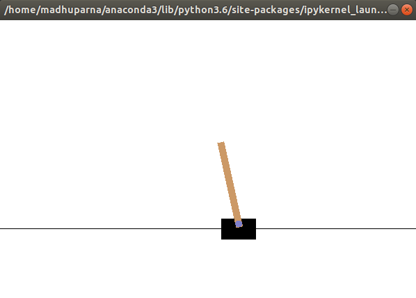
return self.fc(x.contiguous().view(x.size(0), -1))3.We will be using the Cartpole environment from gym.
env = gym.make('CartPole-v0').unwrapped
env.reset()
And use two networks to train the model, policy network which we will update and predict the Q-values, and target network to get the target Q-values for updates and reset the weights of the target network to the policy network’s weight after every 100 episodes.
policy=model()
target_net=model()
target_net.load_state_dict(policy.state_dict())
target_net.eval()
We will use RMSprop optimizer and SmoothL1Loss to train our model.
optimizer = optim.RMSprop(policy.parameters())
criterion = F.smooth_l1_loss
Set the size of replay buffer to 10000, and set gamma the discount factor to 0.99. For the epsilon-greedy strategy to choose actions, we will start with epsilon = 0.9 and reduce it up to 0.05 with a decay rate of 200.
memory=10000
store=[[dict()] for i in range(memory)]
gamma=0.99
EPS_START = 0.9
EPS_END = 0.05
EPS_DECAY = 200
4.These are helper functions to convert PIL Image to an array and vice versa.
def PIL2array(img):
    return np.array(img.getdata(),np.uint8).reshape(img.size[1], img.size[0], 4)

def array2PIL(arr, size):
    mode = 'RGBA'
    arr = arr.reshape(arr.shape[0]*arr.shape[1], arr.shape[2])
    if len(arr[0]) == 3:
        arr = np.c_[arr, 255*np.ones((len(arr),1), np.uint8)]
    return Image.frombuffer(mode, size, arr.tostring(), 'raw', mode, 0, 1)
5.This function will reduce the size of the image to 84 X 84, as it is not feasible to train with such large images.
def processScreen(screen):
    s=[600,400]
    image= array2PIL(screen,s)
    newImage = image.resize((84, 84))
    xtt=PIL2array(newImage)
    xtt=xtt.reshape(xtt.shape[2],xtt.shape[0],xtt.shape[1])
    img=torch.from_numpy(np.array(xtt))
    img=img.type('torch.FloatTensor')
    return img/255.0
6.Here we are adding the episodes to the memory, for each state in memory we are storing its next state, reward, and action taken at that state.
def addEpisode(ind,prev,curr,reward,act):
    if len(store[ind]) ==0:
        store[ind][0]={'prev':prev,'curr':curr,'reward':reward,'action':act}
    else:
        store[ind].append({'prev':prev,'curr':curr,'reward':reward,'action':act})
7.In this function, we will implement the central training part. So, we start with selecting an episode randomly from memory. We will use the Sequential update here, i.e., train on the entire episode from the start till the end. Next, we get the target values from the target network and update the policy network.
def trainNet(total_episodes):
    if total_episodes==0:
        return
    ep=random.randint(0,total_episodes-1)
    if len(store[ep]) < 8:
        return
    else:
        start=random.randint(1,len(store[ep])-1)
        length=len(store[ep])
        inp=[]
        target=[]
        rew=torch.Tensor(1,length-start)
        actions=torch.Tensor(1,length-start)

        for i in range(start,length,1):
            inp.append((store[ep][i]).get('prev'))
            target.append((store[ep][i]).get('curr'))
            rew[0][i-start]=store[ep][i].get('reward')
            actions[0][i-start]=store[ep][i].get('action')
        targets = torch.Tensor(target[0].shape[0],target[0].shape[1],target[0].shape[2])
        torch.cat(target, out=targets)
        ccs=torch.Tensor(inp[0].shape[0],inp[0].shape[1],inp[0].shape[2])
        torch.cat(inp, out=ccs)
        hidden = policy.init_hidden(length-start)
        qvals= target_net(targets,hidden)
        actions=actions.type('torch.LongTensor')
        actions=actions.reshape(length-start,1)
        hidden = policy.init_hidden(length-start)
        inps=policy(ccs,hidden).gather(1,actions)
        p1,p2=qvals.detach().max(1)
        targ = torch.Tensor(1,p1.shape[0])
        for num in range(start,length,1):
            if num==len(store[ep])-1:
                targ[0][num-start]=rew[0][num-start]
            else:
                targ[0][num-start]=rew[0][num-start]+gamma*p1[num-start]
        optimizer.zero_grad()
        inps=inps.reshape(1,length-start)
        loss = criterion(inps,targ)
        loss.backward()
        for param in policy.parameters():
            param.grad.data.clamp(-1,1)
        optimizer.step()
8.Now, we will implement the algorithm. At the beginning of every episode, we reset the environment and continue until the environment returns done = True. We render the environment once before taking action and then after taking action. And store them along with reward received and action in the memory. We use the epsilon-greedy strategy to select the action, in Cartpole environment there are just two possible actions left or right.
def trainDRQN(episodes):
    steps_done=0
    for i in range(0,episodes,1):
        print("Episode",i)
        env.reset()
        prev=env.render(mode='rgb_array')
        prev=processScreen(prev)
        done=False
        steps=0
        rew=0
        while done == False:
            eps_threshold = EPS_END + (EPS_START - EPS_END) * \
            math.exp(-1. * steps_done / EPS_DECAY)
            print(steps,end=" ")
            steps+=1
            hidden = policy.init_hidden(1)
            output=policy(prev.unsqueeze(0),hidden)
            action=(output.argmax()).item()
            rand= random.uniform(0,1)
            if rand < 0.05:
                action=random.randint(0,1)

            _,reward,done,_=env.step(action)
            rew=rew+reward
            if steps>200:
                terminal = torch.zeros(prev.shape[0],prev.shape[1],prev.shape[2])
                addEpisode(i,prev.unsqueeze(0),terminal.unsqueeze(0),-10,action)
                f=0
                break
            sc=env.render(mode='rgb_array')
            sc=processScreen(sc)
            addEpisode(i,prev.unsqueeze(0),sc.unsqueeze(0),reward,action)
            trainNet(i)
            prev=sc
            steps_done+=1
        terminal = torch.zeros(prev.shape[0],prev.shape[1],prev.shape[2])
        print(rew)
        addEpisode(i,prev.unsqueeze(0),terminal.unsqueeze(0),-10,action)
        if i%10==0:
            target_net.load_state_dict(policy.state_dict())
9.Start training!
trainDRQN(2000)