Introduction to Q-learning!
In this article, we will learn about Q-learning and implement the algorithm from scratch. We will also make our own small board game to test the algorithm.
What is Q-learning
Q-learning is an off-policy and model-free Reinforcement Learning algorithm. Model-free means that we need not know the details of the environment i.e how and with what probability the next state is being generated, given current state and action. And off-policy means action-value function, Q, directly approximates the optimal action-value function, independent of the policy being followed.
Setting up the environment
Let us start by defining a simple problem and then we will see how it can be solved using Q-learning. Consider a simple board game, a board with a Start cell and a Goal cell. We can also add a blocked cell to our board. Now, the goal is to learn a path from Start cell represented by S to Goal Cell represented by G without going into the blocked cell X.
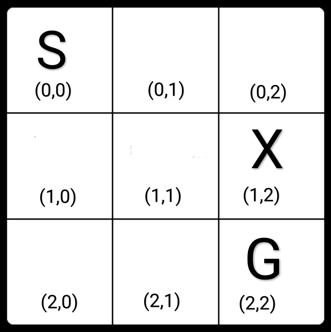
The possible actions from each state are:
1.UP
2.DOWN
3.RIGHT
4.LEFT
Let’s set the rewards now,
1.A reward of +10 to successfully reach the Goal(G).
2.A reward of -10 when it reaches the blocked state.
3.A reward of -1 for all other actions.
Why do you think we define the rewards in this way?
Well +10 for the Goal obviously because that is a desirable state and our algorithm aims at maximizing the reward, so it should get a good amount of reward for completing the task.
And we don’t want to bump into those blocked states so we set the reward for those states to be -10 so that our algorithm learns to not go to those states.
And a reward of -1 for taking any other action because we want to find the shortest way from the Start position to the Goal, we don’t want to just wander around unnecessarily. But what if we set the reward to +1 for every successful step?
Well then our algorithm will learn to maximize the reward just by wandering around that is now it can keep moving between cell (0,1) and cell (1,0) and get +1 for every step and thus maximizing the reward without reaching the Goal! But when the reward is -1 it is being punished for every extra step and thus it will learn to take the shortest path from Start to Goal. Therefore choosing rewards carefully is important.
Let’s write the code for this game
def game(state,action):
	#Awarding 10 for reaching the goal
	if state[0]==2 and state[1]==1 and action==3:
			return [10,[2,2]]
	# -10 for bumping into the blocked state
	elif state[0]==1 and state[1]==1 and action==3:
			return [-10,[1,1]]
	# -10 for bumping into the blocked state
	elif state[0]==0 and state[1]==2 and action==2:
			return [-10,[0,2]]
	#For all other actions -1 reward
	else:
		if action==1:
			x=state[0]-1
			y=state[1]
			if x<0:
				x=0
			return [-1,[x,y]]
		elif action == 2:
			x=state[0]+1
			y=state[1]
			if x>2:
				x=2
			return [-1,[x,y]]
		elif action ==3:
			x=state[0]
			y=state[1]+1
			if y>2:
				y=2
			return [-1,[x,y]]
		else:
			x=state[0]
			y=state[1]-1
			if y<0:
				y=0
			return [-1,[x,y]]
Q-Learning Algorithm
In the Q-learning algorithm, we learn the Q-value for the actions taken from a state. Q-value of an action is basically the expected future reward we can get if that action is taken from the current state.
Here is the discount factor and is the Reward at time step t+1 and so on.
The Q-function takes two inputs state and action and returns the expected future reward. In this algorithm, we experience the environment again and again like playing the game several times, every time an action is taken we update its Q-value which was set randomly initially. The update is performed according to the following equation :
Here is the learning rate and is the discount factor.
Next, to select an action from a given state we use the epsilon-greedy strategy.
Epsilon-Greedy Strategy
In this, we select the action with maximum Q-value with a probability of 1- and select a random action with a probability of . This is used to balance exploration and exploitation. While implementing we generate a random number, if this number is greater than , then we will do exploitation i.e select the best action, and if it is less than we select an action randomly from that state thus exploring.
Let’s implement the algorithm in 3 steps
Step 1. Set the hyperparameters and initialize the Q-table( the table consisting the Q-values of the actions)
def main():
	#Set the Learning rate
	alpha=0.2
	epsilon=0.2
	#Set the discount factor
	discount=0.9
	#Create an empty table which will hold the Q-value for each action in every state
	#e.g Qvalue[1][2] stores a list of 4 values corresponding to the 4 actions from state (1,2)
	Qvalue=[[[] for x in range(3)] for y in range(3)]
	for i in range(3):
		for j in range(3):
			# For terminal state set the Q-values to 0
			if i==2 and j==2:
				Qvalue[i][j][:]= [0,0,0,0]
			#For all other states set the Q-values to random integers
			else:
				Qvalue[i][j][:]= random.sample(range(5), 4)
Step 2. Play the game several times and update the Q-table.
#Set the number of games
numgames=100
for i in range(numgames):
	#Starting with state (0,0)
	state=[0,0]
	#Loop untill terminal state
	while state!=[2,2]:
		#Generate a random number between 0 and 1
		randomnum= random.uniform(0,1)
		action=0
		#Choose the best action if the random number is greater than epsilon
		if randomnum>=epsilon:
			lst=Qvalue[state[0]][state[1]]
			action=lst.index(max(lst))+1
		#Else choose an action randomly
		else:
			action=random.randint(1,4)

		#Play the game
		#The game method will return the reward and next state
		reward,nextstate = game(state,action)
		#nxtlist stores the Qvalue of the actions from the nextstate
		nxtlist=Qvalue[nextstate[0]][nextstate[1]]
		#currval is the Q-value of the action taken in this step
		currval=Qvalue[state[0]][state[1]][action-1]
		#Update the Q-value according to the equation
		Qvalue[state[0]][state[1]][action-1]= currval +  alpha * ( reward + discount*(max(nxtlist)) - currval)
		state=nextstate
Step 3. Print the Q-values learned, play the final game and observe the actions taken
	print("Qvalues after playing ",numgames," games :")
	print("	    	Actions")
	print("		UP DOWN RIGHT LEFT")
	for i in range(3):
		for j in range(3):
			print("State (",i,",",j,") :",end="")
			for k in range(4):
				print(round(float(Qvalue[i][j][k]),1),end="   ")
			print(" ")
	print()
	#Playing the game by choosing action with max Qvalue from each state encountered
	print("Playing Game :")
	state=[0,0]
	totalreward=0
	print("State[0,0] --->",end=" ")
	while state!=[2,2]:
		lst=Qvalue[state[0]][state[1]]
		action=lst.index(max(lst))+1
		reward,nxtstate=game(state,action)
		totalreward=totalreward+reward
		state=nxtstate
		print("State[",state[0],",",state[1],"] --->",end=" ")

	print("Total reward = ",totalreward)
Now run this code and observe the output:
Qvalues after playing  100  games :
	    	Actions
		UP DOWN RIGHT LEFT
State ( 0 , 0 ) :1.7   2.9   4.6   2.5
State ( 0 , 1 ) :3.5   6.2   1.0   0.6
State ( 0 , 2 ) :0.4   -2.7   0.8   3.5
State ( 1 , 0 ) :0.8   1.1   5.9   1.3
State ( 1 , 1 ) :3.7   8.0   -2.8   2.9
State ( 1 , 2 ) :2.0   4.0   0.0   1.0
State ( 2 , 0 ) :0.7   0.5   5.6   0.8
State ( 2 , 1 ) :4.2   5.7   10.0   1.6
State ( 2 , 2 ) :0.0   0.0   0.0   0.0

Playing Game :
State[0,0] ---> State[ 0 , 1 ] ---> State[ 1 , 1 ] ---> State[ 2 , 1 ] ---> State[ 2 , 2 ] ---> Total reward =  7
Next, we will change the hyper parameters and see the effects.
Analyzing the effects of Hyperparameters
1. Number of games
Observe that the path learned by our algorithm after playing 100 games is this:
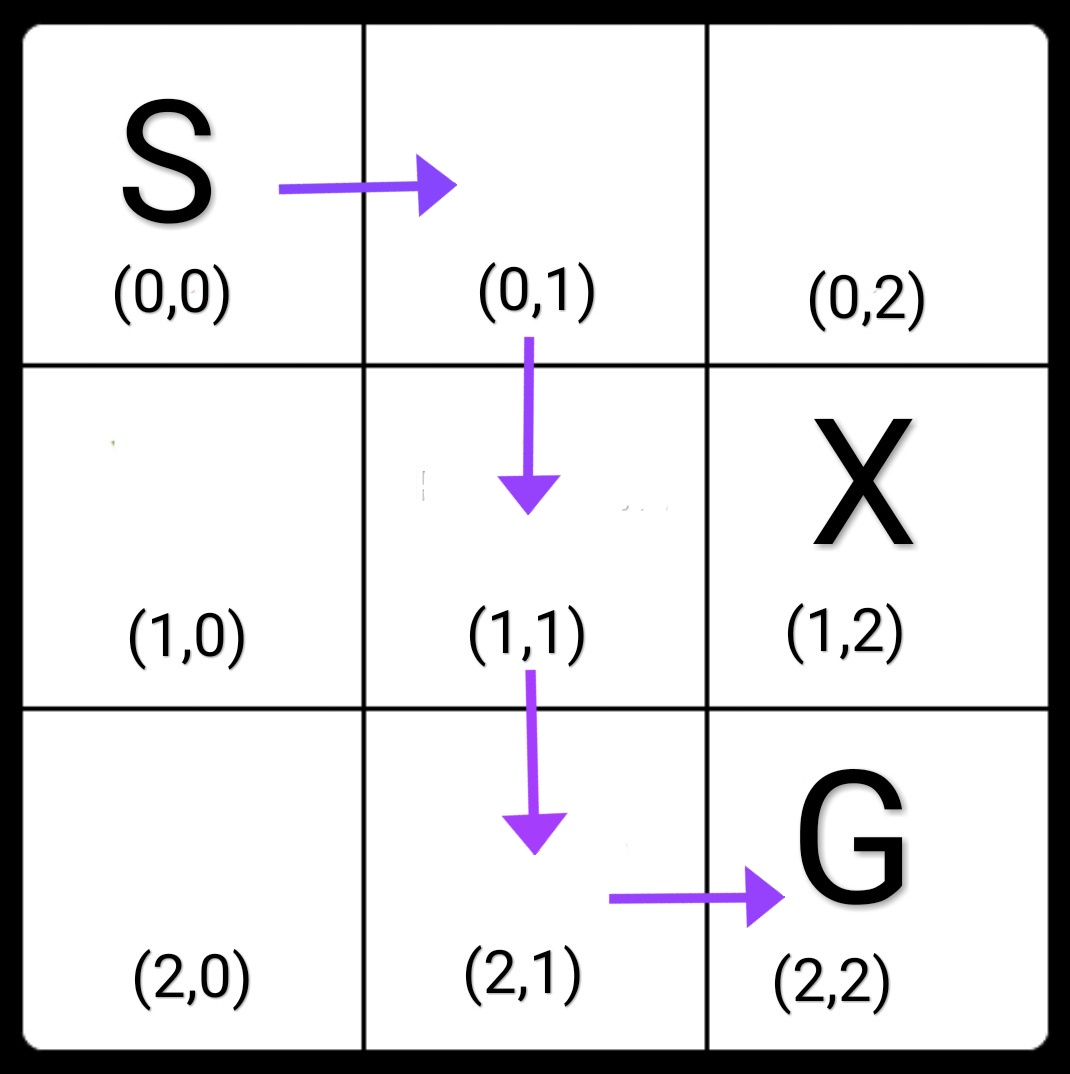
Is this the best way to go from Start to Goal?
We see that currently our algorithm is taking a path that goes through cell (1,1) which is closer to the blocked cell (1,2), i.e this is not the safest path to go from Start to Goal. Now change the parameter numgames from 100 to 1000, and let’s see if the agent learns something better after playing 1000 games. This is the output :
Qvalues after playing  1000  games :
	    	Actions
		UP DOWN RIGHT LEFT
State ( 0 , 0 ) :3.1   4.6   4.4   3.1
State ( 0 , 1 ) :0.7   6.2   1.5   3.1
State ( 0 , 2 ) :3.0   2.0   0.0   3.2
State ( 1 , 0 ) :3.1   6.2   6.2   4.6
State ( 1 , 1 ) :3.2   8.0   -2.9   4.6
State ( 1 , 2 ) :1.0   4.0   3.0   0.0
State ( 2 , 0 ) :4.6   6.2   8.0   6.2
State ( 2 , 1 ) :6.2   8.0   10.0   6.2
State ( 2 , 2 ) :0.0   0.0   0.0   0.0

Playing Game :
State[0,0] ---> State[ 1 , 0 ] ---> State[ 2 , 0 ] ---> State[ 2 , 1 ] ---> State[ 2 , 2 ] ---> Total reward =  7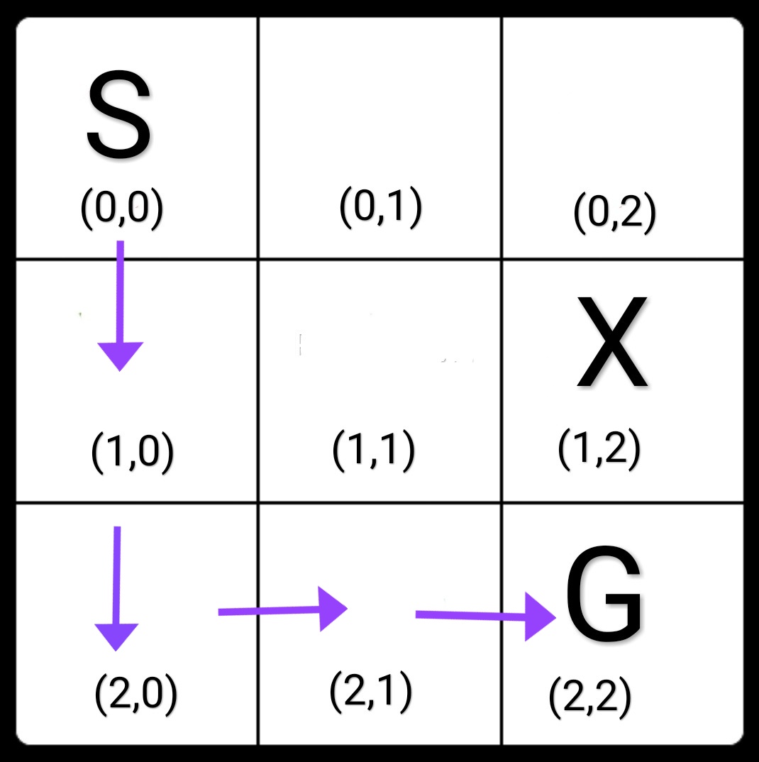
Now we see that it has learned a safer path from S to G, thus avoiding the Blocked cell and staying as far as possible from it!
2. Learning Rate
The learning rate or step size determines to what extent newly acquired information overrides old information. A factor of 0 makes the agent learn nothing (exclusively exploiting prior knowledge), while a factor of 1 makes the agent consider only the most recent information (ignoring prior knowledge to explore possibilities).
3.Discount Factor
The discount factor determines the importance of future rewards. A factor of 0 will make the agent “myopic” (or short-sighted) by only considering current rewards, i.e. (in the update rule), while a factor approaching 1 will make it strive for a long-term high reward. If the discount factor meets or exceeds 1, the action values may diverge. For = 1 , without a terminal state, or if the agent never reaches one, all environment histories become infinitely long, and utilities with additive, undiscounted rewards generally become infinite.
4.Epsilon
When the value of epsilon is too small, then with a small probability the algorithm chooses random actions or explores. It will choose the best action i.e exploit most of the time as probability corresponding to that is high for smaller values of epsilon. If it is set to a high value then the agent will explore more.